Ratings sites – like Rotten Tomatoes and IMDb for movies or Goodreads for books – are annoying. They each seem to have their norms where the same rating means different things on different sites. A rating of 60% on one site might be good, but 6/10 (equivalent to 60%) on another site might be terrible. So you need to do some extra mental work to set your expectations based on the specific site you’re on.
Ratings also often don’t use their full scale. If you’ve bought something from Amazon, you’re probably familiar with this. The theoretical lower bound of ratings might be 1 star, but in reality, ratings rarely go below 3 stars. So you need to do a second bit of extra mental work to re-calculate the fact that “3 stars” really means “1 star”.
Sometimes you do see an item with an unambiguously good or bad score, like 5 stars or 1 star…but then you see that only one or two people have rated it. So you need to do a third bit of extra mental work to take number of ratings into account, since an item with 4.8 stars and 10,000 ratings is probably better than an item with 5.0 stars and 2 ratings.
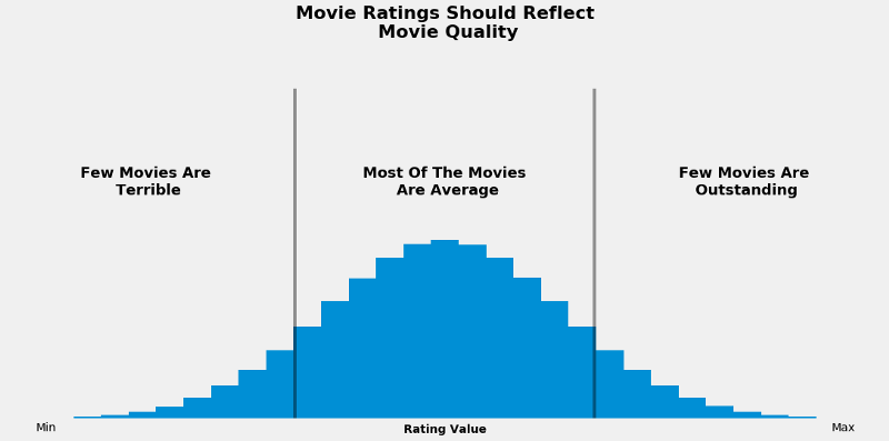
The article Whose ratings should you trust? by Alex Olteanu does a good job of capturing my frustration. I want ratings to look like this:
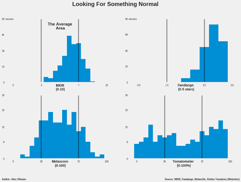
But ratings actually look like this:
In a two-post series, I will “fix” some of these ratings problems:
- Address items with few ratings by using empirical Bayes estimation to estimate more reasonable ratings (this post)
- Normalizing and rescaling ratings so that they are easier to interpret (and look more like that nice, symmetrical normal curve pictured above) (link to post)
Setup
First, we’ll load our packages and import the data. We’re going to use a dataset set of about 9,000 children’s books that have been rated from 1-5 stars. In terms of packages, in addition to the tidyverse, we’ll use:
scalesfor nicely-formatted numbers and useful re-scaling functionsstats4andbroomto help us with our empirical Bayes estimationextrafontandfishualizeto make our graphs look nicegganimateto visualize what exactly empirical Bayes estimation does to the ratingsknitrandkableExtrato get nicely-formatted tables for this post (not necessary if you’re just doing this in RStudio)
library(tidyverse)
library(scales)
library(stats4)
library(broom)
library(extrafont)
library(fishualize)
library(gganimate)
library(knitr)
library(kableExtra)

theme_set(theme_light())

books <- read_tsv("https://raw.githubusercontent.com/tacookson/data/master/childrens-book-ratings/childrens-books.txt") %>%
  # Select only fields we're using (isbn, title, author, and ratings)
  select(isbn:author, rating:rating_1)
We’re not doing any exploratory data analysis or feature engineering, so our data is simple: the book’s ISBN and title, the author, the raw overall rating, and the number of people who rated the book at each star level:
# For reproducability
set.seed(7829)

books %>%
  sample_n(6) %>%
  kable(format = "html") %>%
kable_styling()| isbn | title | author | rating | rating_count | rating_5 | rating_4 | rating_3 | rating_2 | rating_1 |
|---|---|---|---|---|---|---|---|---|---|
| 1495328481 | Calamity Chick: Moves away ! | Olivier Toppin | 4.80 | 5 | 4 | 1 | 0 | 0 | 0 |
| 194130267X | Sheets | Brenna Thummler | 3.76 | 10933 | 2997 | 3743 | 3097 | 763 | 333 |
| 0689829531 | Olivia | Ian Falconer | 4.14 | 58456 | 28141 | 15848 | 10290 | 2713 | 1464 |
| 152374720X | Reflecto Girl: Book 1 | Violet Plum (Author) | 5.00 | 17 | 17 | 0 | 0 | 0 | 0 |
| 1423116712 | Mustache! | Mac Barnett, Kevin Cornell | 3.70 | 851 | 205 | 286 | 277 | 68 | 15 |
| 0553524267 | What Pet Should I Get? | Dr. Seuss | 3.80 | 4246 | 1358 | 1275 | 1146 | 353 | 114 |
What do the raw ratings look like?
Before fixing the ratings, we need to know what we’re fixing! Let’s look at the distribution of ratings:
books %>%
  filter(!is.na(rating)) %>%
  ggplot(aes(rating)) +
  geom_histogram(binwidth = 0.1, fill = "#461220", alpha = 0.8) +
  expand_limits(x = 1) +
  labs(title = "Empirically, an \"average\" book has a 4-star rating",
       subtitle = "And almost no books have fewer than 3 stars",
       x = "Star rating",
       y = "Number of books") +
  theme(text = element_text(family = "Bahnschrift"),
        plot.title = element_text(size = 18),
        axis.text = element_text(size = 16))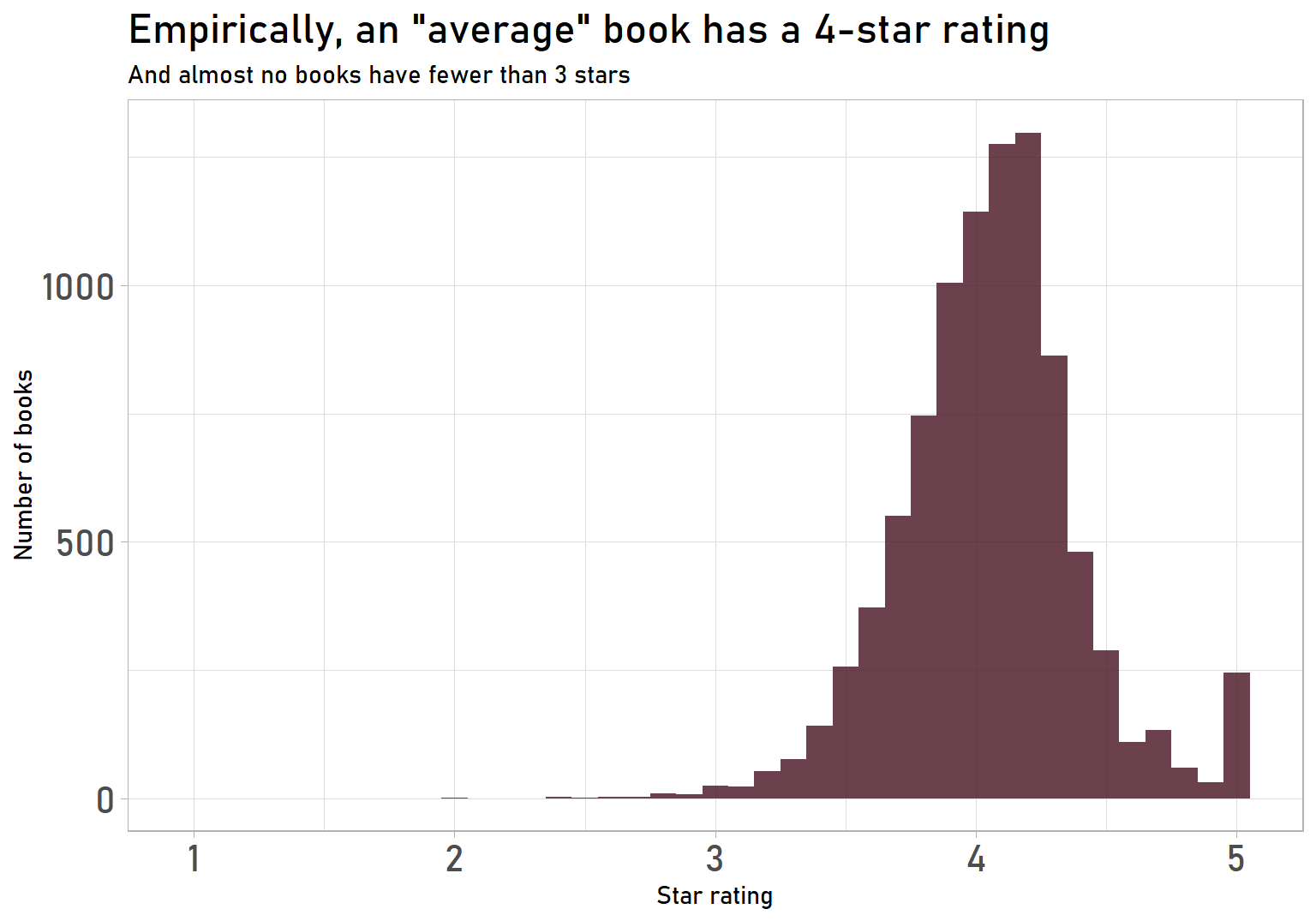
This is fairly typical of crowd-sourced ratings:
- Spike at the maximum 5-star rating
- Ratings concentrated in one part of the range, with almost all books between 3 and 5 stars
- High average rating, with a mean of 4.06 stars
I find that all three issues come up in rating systems like this, but let’s focus on point 1 for now. What are these amazing 5-star books? Let’s look at one:
# For reproducability
set.seed(1867)

# There are many 5-star books, so we will use sample_n() to get just one
books %>%
  select(title, author, rating:rating_1) %>%
  filter(rating == 5) %>%
  sample_n(1) %>%
  kable(format = "html") %>%
kable_styling()| title | author | rating | rating_count | rating_5 | rating_4 | rating_3 | rating_2 | rating_1 |
|---|---|---|---|---|---|---|---|---|
| Pickles and Cake | Laurie S. Johnson (Author) | 5 | 3 | 3 | 0 | 0 | 0 | 0 |
One of them is a book called Pickles and Cake. This could be an amazing book – three people liked it enough to give it a 5-star rating. But how does it stack up against books where more people have weighed in? Let’s compare it to the top-rated book with at least, say, 10,000 ratings:
books %>%
  select(title, author, rating:rating_1) %>%
  filter(rating_count >= 1e4) %>%
  top_n(1, wt = rating) %>%
  kable(format = "html") %>%
kable_styling()| title | author | rating | rating_count | rating_5 | rating_4 | rating_3 | rating_2 | rating_1 |
|---|---|---|---|---|---|---|---|---|
| It’s a Magical World | Bill Watterson | 4.76 | 25572 | 20580 | 3979 | 905 | 63 | 45 |
That book is It’s a Magical World by the peerless Bill Watterson, creator of Calvin & Hobbes, with a rating of 4.76. It has a lower rating than Pickles and Cake’s 5 stars, so is Pickles and Cake the better book? Possibly, but I’m hesitant to make that conclusion. It’s a Magical World has more than 20,000 5-star ratings, while Pickles and Cake has three. I’d want to see more people to weigh in on Pickles and Cake before making that call.
So we need more data to make a judgement about Pickles and Cake. But we don’t have more data. This illustrates a variation of the cold start problem, a common issue when building recommendation engines: a new book will have few or no ratings, so we can’t decide whether it’s good, bad, or average.
We could wait for more ratings to roll in, but this approach has two issues. First, we’d need to set a threshold for how many ratings is “enough”, which is kind of arbitrary. Second, by setting a threshold, we would be ignoring useful data that we have about a book until it reaches that threshold. Say we decide that books need 100 ratings before we trust the star rating. If a book had 99 ratings, we’d say to ourselves, “Welp, no idea what to think about this one!” But we have more information on a book with 99 ratings than a book with 10 ratings. Or a book with 0 ratings.
Fortunately, statistics can help us. We can initially assume a book is average until we get enough data to suggest otherwise. There are two important pieces to that sentence:
- We can initially assume a book is average…: This initial assumption is a Bayesian prior, which is what we believe before we have any data. If I learned of a new book and knew literally nothing about it, I wouldn’t assume it’s amazing or terrible. I’d assume it’s average until I learned more about it. (For a fun introduction to the topic, check out Will Kurt’s excellent blog post Han Solo and Bayesian Priors.)
- …until we get enough data to suggest otherwise: The initial assumption is just that – an initial assumption. As more people rate a book, we’ll start to trust those ratings more than our assumption. As a book gets more and more ratings, our initial assumption will have less influence on what we think a book’s true rating is.
This entire approach is called shrinkage, which David Robinson defines very well in Introduction to Empirical Bayes:
[Shrinkage is] the process of moving all our estimates towards the average. How much it moves these estimates depends on how much evidence we have: if we have very little evidence [like three ratings for Pickles and Cake] we move it a lot, if we have a lot of evidence [like 20,000 ratings for It’s a Magical World] we move it only a little. That’s shrinkage in a nutshell: Extraordinary outliers require extraordinary evidence.
Determining the Bayesian prior
(Note: It will help if you know about the beta and binomial distributions, since what we are about to do is an extension of those ideas. If you’re not familiar, you’ll probably still get the gist, but might find some background research useful. Will Kurt’s blog post Working with Probability Distributions and David Robinson’s blog post Understanding the beta distribution (using baseball statistics) are great primers.)
Distribution of star ratings
We already looked at the distribution of the overall rating, but to determine our prior, we’ll need to understand the distribution of ratings for each star level. Specifically, we’re going to look at the percent of a book’s ratings that are at each level.
Why is that important? It turns out that the distribution of ratings at each star level fits well with the Dirichlet distribution, which describes the range of possible probabilities for multiple outcomes. In our case, these outcomes are 1-star rating, 2-star rating, etc.
If you’re familiar with the beta distribution, the Dirichlet is conceptually similar, except that the Dirichlet can apply to more than two outcomes, whereas the beta distribution applies only to situations with two outcomes. (In fact, the Dirichlet is just the more-than-two-outcomes generalization of the beta distribution. A two-outcome Dirichlet is a beta distribution.)
Again, why is this important? If we look at books with enough ratings that their overall rating has “settled”, fitting a Dirichlet distribution will give us a sense of what a good estimate of the percent of a book’s ratings at each star level will be. Visualizing it will help. These are the distributions for books with at least 500 ratings:
rating_pct <- books %>%
  filter(rating_count > 0) %>%
  mutate_at(vars(rating_5:rating_1), ~ . / rating_count) %>%
  # Filter for books with at least 500 reviews
  filter(rating_count > 500) %>%
  pivot_longer(cols = rating_5:rating_1,
               names_to = "rating_level",
               values_to = "pct_of_ratings") %>%
  # Use Unicode symbol for full star (U+2605) and empty star (U+2606) as facet titles
  mutate(rating_num = parse_number(rating_level),
         stars_label = paste0(strrep("\U2605", rating_num),
                              strrep("\u2606", 5 - rating_num)),
         stars_label = fct_reorder(stars_label, rating_num)) %>%
  select(-rating_num)

rating_pct %>%
  ggplot(aes(pct_of_ratings)) +
  geom_histogram(binwidth = 0.025, fill = "#461220", alpha = 0.8) +
  facet_wrap(~ stars_label, nrow = 1) +
  scale_x_continuous(labels = label_percent()) +
  labs(title = "Proportions of ratings at each star level have their own distributions",
       x = "% of ratings",
       y = "Number of books") +
  theme(text = element_text(family = "Bahnschrift"),
        axis.text = element_text(size = 9),
        strip.text = element_text(size = 20, colour = "black"),
        strip.background = element_blank(),
        panel.grid.minor = element_blank())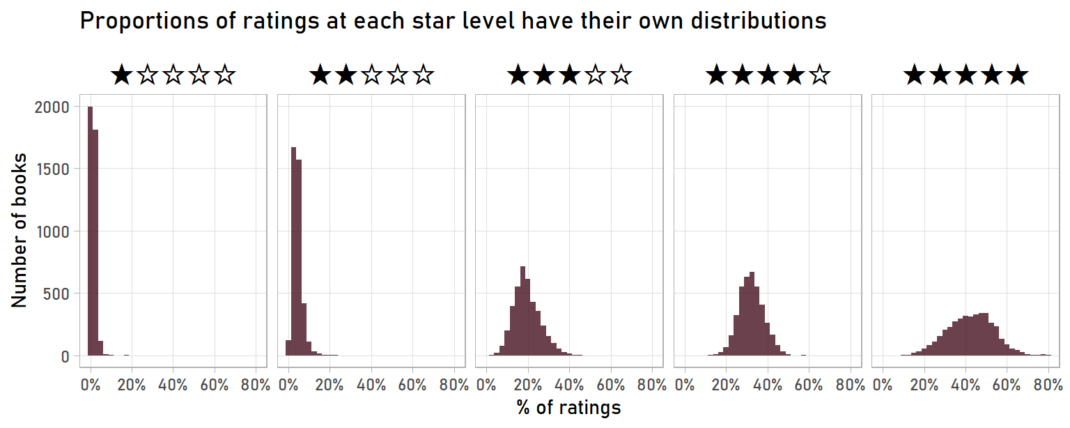
The percent of a book’s ratings at each star level tends toward certain values. For example, 2-star ratings are likely to constitute 0-15% of ratings, while 4-star ratings are likely to constitute 20-50% of ratings. So, if a book got a new rating, we could look at these distributions to get an idea of how likely it is that this new rating will be for 1, 2, 3, 4, or 5 stars (1%, 4%, 20%, 30%, and 45%, respectively).
We can now use this data to fit a Dirichlet-multinomial distribution that will give us an actual number of ratings at each star level instead of a probability for one rating. This, in effect, gives us “starter ratings” to use for each book. So we will treat a book with zero real ratings as having, say, 40 or 50 ratings that start the book off with an average overall rating. This is how our shrinkage works: a book’s first few ratings will be tempered by our “starter ratings”, but as a book gets more real ratings, those real ratings will have more of an effect on the overall rating.
Maximum likelihood estimation of the Dirichlet-Multinomial distribution
We use maximum likelihood estimation (MLE) to estimate the parameters of the Dirichlet-Multinomial distribution using the DirichletMultinomial package. (For an introduction to maximum likelihood estimation, I recommend this StatQuest video by Josh Starmer. I’ll also note that I’m indebted to David Robinson’s already-mentioned book Introduction to Empirical Bayes, which I relied on heavily for the following chunk of code.)
# Create a matrix to feed our MLE of Dirichlet-Multinomial
rating_matrix <- books %>%
  filter(rating_count > 500) %>%
  select(rating_5:rating_1) %>%
  as.matrix()

# Fit a Dirichlet Multinomial distribution
# Input is a matrix of rating counts at each star level
dm_fit <- DirichletMultinomial::dmn(rating_matrix, 1)

# Write a function to tidy DMN object (which dm_fit is)
# (broom's tidy() doesn't work on DMN objects)
# Function from http://varianceexplained.org/r/empirical-bayes-book/
tidy.DMN <- function(x, ...) {
  ret <- as.data.frame(x@fit)
  as_tibble(fix_data_frame(ret, c("conf.low", "estimate", "conf.high")))
}

# Tidy the DMN fit
tidy_dm <- tidy(dm_fit)

# Get parameters into a useful format
par <- tidy_dm %>%
  separate(term, into = c("constant", "rating_stars"), sep = "_", convert = TRUE) %>%
  select(rating_stars,
         prior_ratings = estimate)

# Calculate total prior ratings and mean (used for graphing)
par_total <- sum(par$prior_ratings)
par_mean <- par %>%
  summarise(prior_rating = sum(rating_stars * prior_ratings) / sum(prior_ratings)) %>%
  pull(prior_rating)
The result is a fairly simple dataframe with the number of starter ratings each star level gets:
par %>%
  kable(format = "html") %>%
kable_styling()| rating_stars | prior_ratings |
|---|---|
| 5 | 21.290057 |
| 4 | 16.496105 |
| 3 | 9.838544 |
| 2 | 2.399964 |
| 1 | 1.027657 |
So a book with zero ratings, using our empirical Bayes estimate, will start with 21.29 5-star ratings, 16.50 4-star ratings, etc. (I know it doesn’t make sense to have fractions of ratings, but we’re not talking about real ratings – we can still calculate an overall rating with fractions.)
Overall, our prior gives us about 51 “starter ratings” and an overall rating of 4.07 stars. Again, this will change as a book gets real ratings, but we’ll be less likely to find ourselves in a Pickles and Cake situation where a few good ratings skyrockets a book up to a perfect 5-star rating.
Here’s what the Dirichlet fits from MLE look like (light blue curves) compared to the actual distribution of ratings (red histograms):
dirichlet_density <- tidy_dm %>%
  select(rating_level = term, estimate) %>%
  crossing(pct_of_ratings = seq(0, 0.8, by = 0.0125)) %>%
  mutate(density = dbeta(pct_of_ratings, estimate, par_total - estimate)) %>%
  # Use Unicode symbol for full star (U+2605) and empty star (U+2606) as facet titles
  mutate(rating_num = parse_number(rating_level),
         stars_label = paste0(strrep("\U2605", rating_num),
                              strrep("\U2606", 5 - rating_num)),
         stars_label = fct_reorder(stars_label, rating_num)) %>%
  select(-rating_num)

rating_pct %>%
  ggplot(aes(pct_of_ratings)) +
  geom_histogram(aes(y = ..density..), binwidth = 0.025, fill = "#461220", alpha = 0.8) +
  geom_area(data = dirichlet_density, aes(y = density), fill = "#778DA9", alpha = 0.7) +
  facet_wrap(~ stars_label, nrow = 1) +
  scale_x_continuous(labels = label_percent()) +
  labs(title = "Maximum-Likelihood Estimates fit the data fairly well",
       subtitle = "Red histogram = Actual distribution | Blue curve = MLE fit",
       x = "% of ratings",
       y = "Density") +
  theme(text = element_text(family = "Bahnschrift"),
        axis.text = element_text(size = 9),
        strip.text = element_text(size = 20, colour = "black"),
        strip.background = element_blank(),
        panel.grid.minor = element_blank(),
        panel.grid.major = element_blank())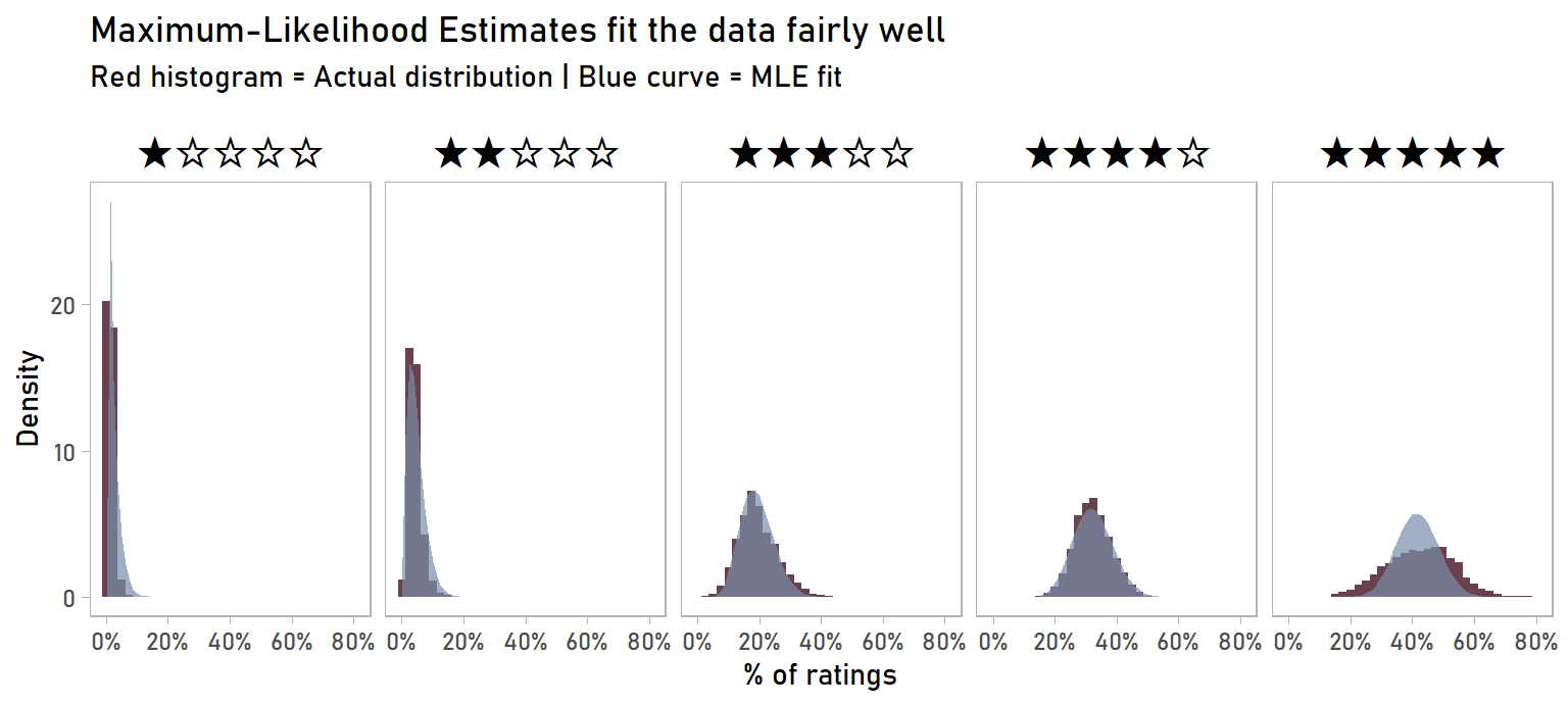
The MLE fit tracks closely to the empirical distribution, so the overall fit is pretty good. One area where the fit isn’t great is the distribution of 5-star ratings: our MLE fit has under-estimated the variance. You can tell this by the MLE blue curve being narrower and taller than the empirical distribution. Even though it’s not perfect, I’m making the call that it’s good enough to use for our shrinkage purposes.
Incorporating the prior into ratings
We can finally calculate the shrunk ratings. We just need need to add the prior “starter ratings” to each book’s existing real ratings.
# Calculate empirical Bayes rating using our prior
books_eb <- books %>%
  pivot_longer(rating_5:rating_1,
               names_to = c("rating_stars"),
               names_pattern = "rating_(.*)",
               names_transform = list(rating_stars = as.integer),
               values_to = "ratings") %>%
  left_join(par, by = "rating_stars") %>%
  group_by(isbn, title, author, rating_count) %>%
  # Calculate original rating from scratch because rating field truncates after two decimal places
  summarise(rating_calc = sum(rating_stars * ratings) / sum(ratings),
            rating_eb = sum(rating_stars * (ratings + prior_ratings)) / sum(ratings + prior_ratings)) %>%
  ungroup()
And we end up with an adjusted rating for each book (rating_eb). Here are the top 10 books, according to our empirical Bayes estimate:
books_eb %>%
  select(-isbn, -rating_calc) %>%
  top_n(10, wt = rating_eb) %>%
  arrange(desc(rating_eb)) %>%
  kable(format = "html") %>%
kable_styling()| title | author | rating_count | rating_eb |
|---|---|---|---|
| 100 Fun Bible Facts: The Exciting way to Learn (100 Bible Facts Book 1) | Ginger Baum | 478 | 4.893236 |
| Jubal’s Field Trip To Heaven: Jubal and Chanan Enter Through the Narrow Gate (Jubal’s Divine Adventures #1) | Ginger Baum | 382 | 4.874187 |
| It’s a Magical World | Bill Watterson | 25572 | 4.757816 |
| There’s Treasure Everywhere | Bill Watterson | 19516 | 4.747868 |
| The Indispensable Calvin and Hobbes | Bill Watterson | 19235 | 4.736054 |
| The Authoritative Calvin and Hobbes: A Calvin and Hobbes Treasury | Bill Watterson | 20598 | 4.733524 |
| Homicidal Psycho Jungle Cat | Bill Watterson | 17584 | 4.720359 |
| A Day in the Life of Marlon Bundo | Jill Twiss (Author), E.G. Keller (Illustrator) | 13375 | 4.718943 |
| The Days Are Just Packed | Bill Watterson | 22159 | 4.693765 |
| The Undefeated | Kwame Alexander, Kadir Nelson (Illustrator) | 2988 | 4.687572 |
Immediately, I’m more confident in these ratings than the originals, which had a bunch of books with 2 or 3 ratings that just happened to be 5 stars. Visually, this is what shrinkage did:
# Format data properly for animation
books_shrunk <- books_eb %>%
  filter(rating_count > 0) %>%
  select(isbn:author, rating_count, rating_calc, rating_eb) %>%
  pivot_longer(rating_calc:rating_eb, names_to = "rating_type", values_to = "rating") %>%
  mutate(rating_type = ifelse(rating_type == "rating_calc", "Original Rating", "Empirical Bayes Rating"))

# Create base plot
p <- books_shrunk %>%
  filter(rating_count <= 200) %>%
  ggplot(aes(rating_count, rating, col = rating_count)) +
  geom_point(alpha = 0.4, size = 0.5) +
  geom_hline(yintercept = par_mean,
             lty = 2,
             size = 0.8,
             col = "red") +
  scale_colour_fish(option = "Ostracion_whitleyi") +
  scale_x_continuous(breaks = seq(0, 200, by = 25)) +
  labs(subtitle = paste0("Dashed line shows Bayesian prior for a book with 0 ratings",
                        "\n",
                        "(Only books with 200 ratings or less shown)"),
       x = "Number of ratings",
       y = "Rating") +
  theme(legend.position = "none",
        text = element_text(family = "Bahnschrift", size = 6),
        plot.title = element_text(size = 8),
        panel.grid.minor.x = element_blank())

# Set animation parameters
anim <- p +
  transition_states(rating_type,
                    transition_length = 1.5,
                    state_length = 1.5) +
  ease_aes("cubic-in-out") +
  ggtitle("{closest_state}")

# Create animation
anim
The books with few ratings – less than 25 – were impact a lot by incorporating a Bayesian prior. But as we get more rating, the prior has less of an effect. You can imagine a book that has 1,000 or 10,000 ratings: our prior will barely move its score.
Before wrapping up, we should note that still need to be careful when interpreting adjusted ratings. They are still susceptible to other forms of statistical bias. For example, the top-rated book is 100 Fun Bible Facts by Ginger Baum. I’m sure it’s an excellent book, but not everyone might consider it excellent. People who took the time to read and rate this book are likely pre-disposed to enjoy books with biblical themes, making this a likely illustration of self-selection bias.
Conclusion
We’ve successfully used empirical Bayes estimation to get more reasonable ratings for our 9,000 children’s books! If you’d like to see the full dataset of adjusted ratings, feel free to download it here. And, if you’re keen to see more adjustments of these ratings, check out the second post of this series, where I normalize and rescale the ratings.